Fama and French Three Factor Model

Properties

tags fin fin/theory

created 15.03.2025, 18:19

modified 08.09.2026, 11:12

published Empty

sources Fama and French Three Factor Model Definition

topics Asset Pricing, Three Factor Model, Factor Investing

authors Jakub

ai-assisted No

Fama and French Three Factor Model Definition:

The Fama and French Three-Factor Model is an asset pricing model that expands on the CAPM by adding size risk and value risk factors to the market risk factor in CAPM. This model considers the fact that value and small-cap stocks outperform markets on a regular basis. By including these two additional factors, the model adjusts for this outperforming tendency, which is thought to make it a better tool for evaluating manager performance.

# Resources

Papers
- The Cross-Section of Expected StockReturns
  - Original Paper
Explainers
- Bogleheads - Fama and French three-factor model ( Link)
  - Bogleheads wiki — clean overview of the model, factors, and comparison vs CAPM
- CFI - Fama-French Three-Factor Model ( Link)
  - Corporate Finance Institute — 2020-01-28, framed for valuation/portfolio performance
- DayTrading - Fama-French 3-5-Factor Model ( Link)
  - 2023-07-15 — covers both 3- and 5-factor variants and ongoing debates
Data
- Kenneth R. French – Data Library (Dartmouth)
  - Provides actual factor time series (MKT-RF, SMB, HML) and the exact portfolio returns used to compute them.
  - Offers detailed documentation on how the factors are constructed from CRSP data.
Videos
- Eugene Fama Why Small Caps and Value Stocks Outperform - ClientInsights
- Fama-French SMB and HML | 6. Calculating Fama-French Factors
  - Wharton lecture
- Is the Value Premium Dead?
  - Explanation why value (factor) premium persists

# Skeptics of Factor Investing

# Factors

Fama and French Three Factor Model Definition:

The Fama and French model has three factors: the size of firms, book-to-market values, and excess return on the market. In other words, the three factors used are small minus big (SMB), high minus low (HML), and the portfolio’s return minus the risk-free rate of return.

# Original Three Factors

(Source: ChatGPT)

Market Factor (MKT - Market Premium)
- Represents the excess return of the market portfolio over the risk-free rate.
- Captures the overall risk and return of the stock market.
- Investors are compensated for taking on systematic market risk.
Size Factor (SMB - Small Minus Big)
- Measures the size premium, where small-cap stocks (companies with a relatively low market capitalization, typically below $2 billion) tend to outperform large-cap stocks over time.
- Based on the idea that smaller companies are riskier but offer higher expected returns.
Value Factor (HML - High Minus Low)
- Captures the value premium, where value stocks (high book-to-market ratio) tend to outperform growth stocks (low book-to-market ratio).
- Value stocks are often considered riskier but offer higher long-term returns.

# High-Level Definition

$$ ER_i = R_f + \beta_i (ER_m - R_f) + s_i \times SMB + h_i \times HML $$

where:

$ER_i$ = Expected return of the investment
$R_f$ = Risk-free rate
$\beta_i$ = Beta of the investment (market risk factor)
$(ER_m - R_f)$ = Market risk premium (same as CAPM)
$SMB$ = Size premium (small minus big)
$HML$ = Value premium (high minus low)
$s_i$ and $h_i$ = Sensitivity coefficients for the SMB and HML factors

# Why Factor Tilt Makes Sense

(Source: ChatGPT)

We expect a higher expected return because we are intentionally taking on additional systematic, non-diversifiable risk — specifically, size and value risk — for which the market pays a premium.

Formally:

$$
\mathbb{E}[R_P] - R_f =
\beta_{P,M}\lambda_M

\beta_{P,SMB}\lambda_{SMB}
\beta_{P,HML}\lambda_{HML}
$$

If $\lambda_{SMB} > 0$ and $\lambda_{HML} > 0$, then increasing exposure to SMB and HML raises expected return only because it raises risk.

No free lunch.

# Risks Of Tilt

Tilting increases exposure to:
- Long periods of underperformance
- Cyclicality
- Deep drawdowns during recessions
Example:
- Value underperformed growth for a full decade (2010s)
- Small caps can lag for very long horizons
So tilting only makes sense if:
- You have a long horizon
- You can stick with the strategy
- You understand why the premium exists

# Video Overview

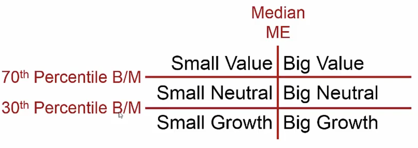
Extremely useful table from the video
Figure

# Definition Deep Dive

(Source: ChatGPT)
The Fama–French Three-Factor Model explains excess returns using three systematic risk factors:
$$
R_{i,t} - R_{f,t}

\alpha_i

\beta_{i,M}(R_{M,t} - R_{f,t})
\beta_{i,SMB},\text{SMB}_t
\beta_{i,HML},\text{HML}_t
\varepsilon_{i,t}
$$
where:
$R_{i,t}$ is the return on asset $i$ at time $t$
$R_{f,t}$ is the risk-free rate
$R_{M,t} - R_{f,t}$ is the market factor
$\text{SMB}_t$ and $\text{HML}_t$ are the size and value factors

# Market Factor (Definition)

The market factor is the excess return on the value-weighted market portfolio of all eligible stocks:
$$
R_{M,t}

\sum_{i \in \mathcal{U}t}
\frac{ME{i,t}}{\sum_{j \in \mathcal{U}t} ME{j,t}}
, R_{i,t}
$$

so that:

$$ \text{MKT}_t = R_{M,t} - R_{f,t} $$

$\mathcal{U}_t$ is the universe of eligible stocks (e.g. NYSE/AMEX/NASDAQ common stocks)
$ME_{i,t}$ denotes market equity
The market factor captures aggregate equity market risk

# 1. Universe and Timing

Let:

$\mathcal{U}_t$: the universe of eligible stocks at time $t$
Portfolios are rebalanced annually (typically end of June)
Returns are measured monthly

Key firm characteristics:

Market Equity (ME) = market capitalization
Book-to-Market (B/M) = book value of equity divided by market equity

# 2. Sorting Procedure (Core Idea)

# Step 1: Size Sort

Stocks are sorted by market equity:

Small (S): bottom 50%
Big (B): top 50%

Formally:

$$ S_t = { i \in \mathcal{U}_t : ME_i \le \text{median}(ME) } $$

$$ B_t = { i \in \mathcal{U}_t : ME_i > \text{median}(ME) } $$

# Step 2: Value Sort

Stocks are sorted by book-to-market into three groups:

Low (L): bottom 30%
Medium (M): middle 40%
High (H): top 30%

$$ L_t, M_t, H_t \subset \mathcal{U}_t $$

# 3. The Six Intersection Portfolios

Portfolio	Definition
SL	Small & Low B/M
SM	Small & Medium B/M
SH	Small & High B/M
BL	Big & Low B/M
BM	Big & Medium B/M
BH	Big & High B/M

Each portfolio is value-weighted:

$$
R_{P,t}

\sum_{i \in P} w_{i,t} R_{i,t},
\quad
w_{i,t}

\frac{ME_{i,t}}{\sum_{j \in P} ME_{j,t}}
$$

# 4. SMB — Small Minus Big

$$
\text{SMB}_t

\frac{1}{3}(R_{SL,t} + R_{SM,t} + R_{SH,t})

\frac{1}{3}(R_{BL,t} + R_{BM,t} + R_{BH,t})
$$

Long small stocks
Short big stocks
Neutral with respect to value

# 5. HML — High Minus Low

$$
\text{HML}_t

\frac{1}{2}(R_{SH,t} + R_{BH,t})

\frac{1}{2}(R_{SL,t} + R_{BL,t})
$$

Long value stocks (high B/M)
Short growth stocks (low B/M)
Neutral with respect to size

# Why the Three Factors Are (Approximately) Independent

The market factor captures aggregate equity risk.
SMB averages small minus big returns within each value group.
HML averages value minus growth returns within each size group.

This construction removes overlapping effects by design, making SMB and HML approximately market-neutral and mutually orthogonal. While not perfectly uncorrelated in finite samples, the factors are empirically distinct and capture separate dimensions of risk.