Layer Normalization

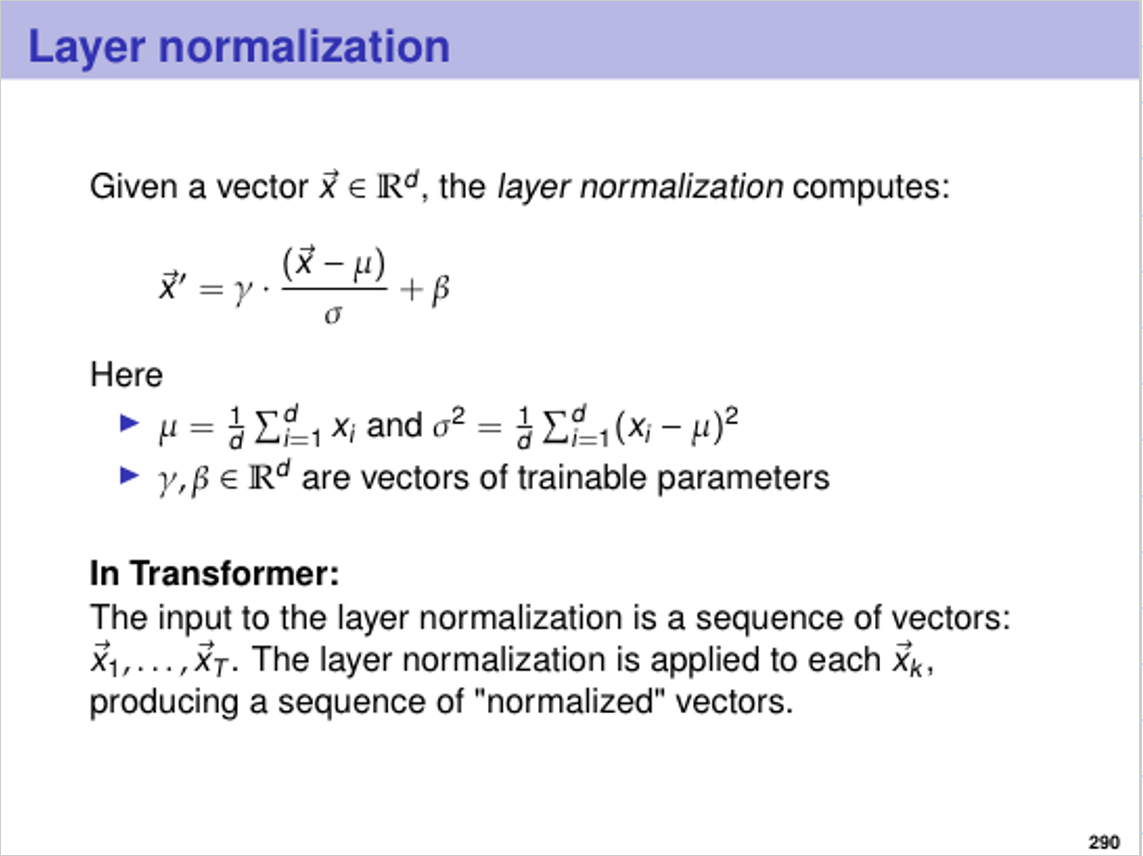
# Definition

Section source: PV021 course

# Backpropagation and Gradients Computation:

Section source: ChatGPT¹

During backpropagation, the goal is to compute how the loss \(L\) changes with respect to each parameter involved in the forward pass, including \(\gamma\), \(\beta\), and the normalized input \(\hat{x}_i\).

# Step 1: Gradient w.r.t. \(\gamma\):

The gradient of the loss \(L\) with respect to \(\gamma\) is computed as follows:

$$ \frac{\partial L}{\partial \gamma} = \sum_{i=1}^{d} \frac{\partial L}{\partial x'_i} \cdot \hat{x}_i $$

Here, \(\frac{\partial L}{\partial x'_i}\) is the gradient of the loss with respect to the output of layer normalization, which comes from the downstream layers during backpropagation. Essentially, we are scaling the backpropagated gradients by the normalized input \(\hat{x}_i\) to compute the gradient for \(\gamma\).

# Step 2: Gradient w.r.t. \(\beta\):

Similarly, the gradient of the loss \(L\) with respect to \(\beta\) is computed as:

$$ \frac{\partial L}{\partial \beta} = \sum_{i=1}^{d} \frac{\partial L}{\partial x'_i} $$

Here, the gradient with respect to \(\beta\) is simply the sum of the gradients of the loss with respect to the outputs \(x'_i\). This makes sense because \(\beta\) is applied as a shift and affects the output directly.

# Step 3: Gradient w.r.t. Normalized Input (\(\hat{x}_i\)):

Next, we compute the gradient with respect to the normalized input \(\hat{x}_i\):

$$ \frac{\partial L}{\partial \hat{x}_i} = \frac{\partial L}{\partial x'_i} \cdot \gamma $$

Here, the gradient is scaled by \(\gamma\) since \(\hat{x}_i\) was multiplied by \(\gamma\) during the forward pass.

# Step 4: Gradient w.r.t. Input (\(x_i\)):

Finally, we need to compute the gradient with respect to the original input \(x_i\). To do this, we need to take into account how \(x_i\) affects \(\hat{x}_i\), which in turn affects the final output. The key here is that \(x_i\) affects both the mean \(\mu\) and the variance \(\sigma^2\), so we need to apply the chain rule to propagate the gradient back through these calculations.

First, the gradient w.r.t. \(x_i\) can be split into three components:

$$ \frac{\partial L}{\partial x_i} = \frac{1}{\sigma} \left( \frac{\partial L}{\partial \hat{x}_i} - \frac{1}{d} \sum_{j=1}^{d} \frac{\partial L}{\partial \hat{x}_j} - \hat{x}_i \cdot \frac{1}{d} \sum_{j=1}^{d} \frac{\partial L}{\partial \hat{x}_j} \cdot \hat{x}_j \right) $$

Here:

• \(\frac{\partial L}{\partial \hat{x}_i}\) is the gradient from step 3.
• The terms involving sums account for the effect of \(x_i\) on the mean \(\mu\) and variance \(\sigma^2\), since all elements of \(\vec{x}\) contribute to these quantities.

This expression accounts for the contribution of \(x_i\) to both the normalization (via the mean and variance) and the final output.