Self-Attention

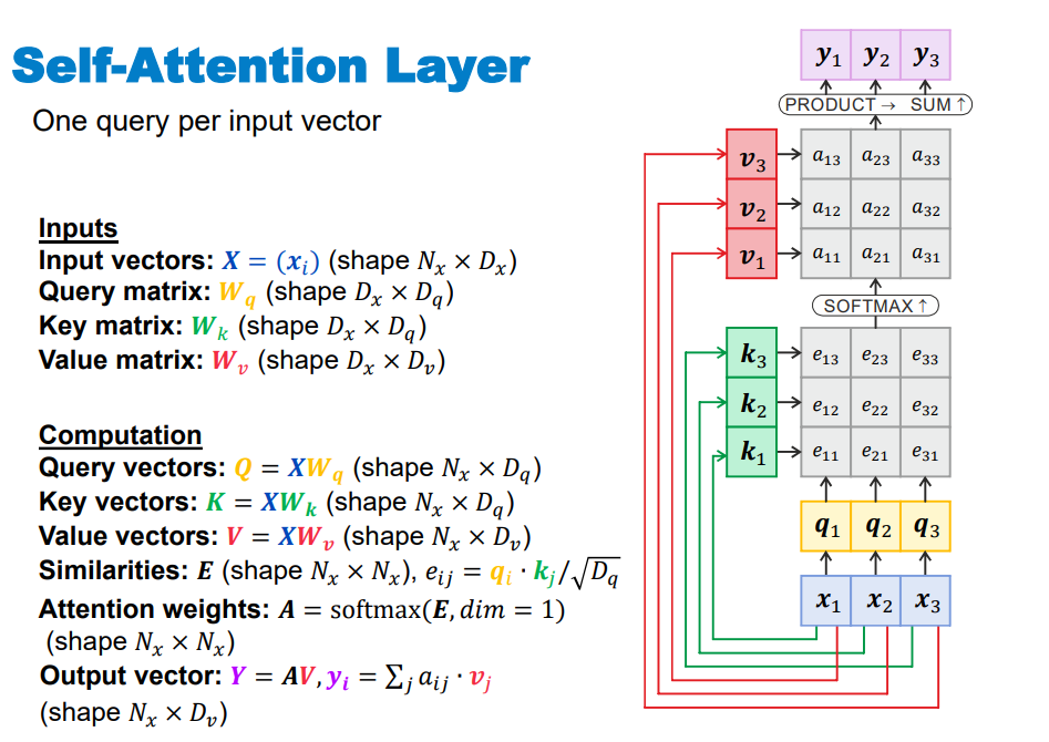
• Source: Understanding Attention Mechanism, Self-Attention Mechanism and Multi-Head Self-Attention Mechanism

# Intuition

• Q/K/V split — each token simultaneously plays three roles through separate learned projections
  • Query (\(\mathbf{Q}\)): “what am I looking for?”
  • Key (\(\mathbf{K}\)): “what do I advertise about myself?”
  • Value (\(\mathbf{V}\)): “what do I actually contribute if selected?”
  • Decoupling matching (\(Q\)/\(K\)) from content (\(V\)) gives the model much more expressive power than a single vector per token
• Dot-product as similarity — \(\mathbf{Q}\mathbf{K}^T\) measures how compatible each query is with every key; a high dot product means “pay attention here”
• \(\sqrt{D_q}\) scaling — in high dimensions the dot products grow proportionally to \(D_q\), which pushes softmax into saturation (near-zero gradients everywhere); dividing by \(\sqrt{D_q}\) keeps the variance of the scores at ~1 and keeps gradients healthy
• Softmax → weighted sum — softmax turns raw compatibility scores into a probability distribution; the output is then a context-aware blend of value vectors rather than a hard selection, allowing the model to “read” information from multiple positions simultaneously

# Modifications

• Masked Self-Attention
  • A variant of self-attention used in autoregressive models (e.g., GPT) where a causal mask is applied to prevent attending to future tokens, ensuring that each position can only attend to past and current positions.
• Multi-head Self-Attention
  • An extension of self-attention where multiple attention heads compute attention scores in parallel on different learned projections of the input, capturing diverse contextual information before concatenating and projecting them back into the original dimension.
• Cross-attention involves using keys and values from the encoder’s output in a separate cross-attention block in the decoder.
• Flash Attention
  • FlashAttention, an IO-aware exact attention algorithm that uses tiling to reduce the number of memory reads/writes between GPU high bandwidth memory (HBM) and GPU on-chip SRAM.
• Multi-Token Attention
  • Multi-Token Attention (MTA), which applies convolution operations across keys, queries, and attention heads, allowing neighboring tokens to influence each other’s attention weights. This approach enables the model to condition its attention on multiple vector pairs simultaneously, facilitating more precise context location in complex scenarios.
• Ghost-Attention
  • Ghost Attention (GAtt), a very simple method inspired by Context Distillation that hacks the fine-tuning data to help the attention focus in a multi-stage process. GAtt enables dialogue control over multiple turns
• LESS IS MORE
  • LESS IS MORE: TRAINING-FREE SPARSE ATTENTION WITH GLOBAL LOCALITY FOR EFFICIENT REASONING
  • We introduce LessIsMore, a training-free sparse attention mechanism for reasoning tasks, which leverages global attention patterns rather than relying on traditional head-specific local optimizations. LessIsMore aggregates token selections from local attention heads with recent contextual information, enabling unified cross-head token ranking for future decoding layers
• Attention Residuals
  • Applies softmax attention not across sequence positions but across depth — each layer attends over all prior layer outputs to selectively aggregate earlier representations, replacing fixed residual skip connections

# Complexity

Number of operations in self-attention scales quadratically with the sequence length \(O(\text{seq\_len}^2)\). A shorter input sequence means a smaller attention matrix and fewer dot products, so the model uses less computation and memory.

For example, with a full-length sequence of size 512, the self-attention would involve 5122^22 = 262,144 operations for the attention matrix, whereas with a sequence length of 300, it would involve only 90,000 operations, significantly reducing the computational load.

# Forward Pass And Backpropagation

# Forward Pass

Given:

• Input vectors: \(\mathbf{X} = [\mathbf{x}_1, \mathbf{x}_2, \mathbf{x}_3]\) with shape \(N_x \times D_x\)
• Query matrix: \(\mathbf{W}_q\) with shape \(D_x \times D_q\)
• Key matrix: \(\mathbf{W}_k\) with shape \(D_x \times D_q\)
• Value matrix: \(\mathbf{W}_v\) with shape \(D_x \times D_v\)

The computations are as follows:

1. Compute Query, Key, and Value vectors:
   

   $$ \mathbf{Q} = \mathbf{X}\mathbf{W}_q \quad (\text{shape } N_x \times D_q) $$

   
   

   $$ \mathbf{K} = \mathbf{X}\mathbf{W}_k \quad (\text{shape } N_x \times D_q) $$

   
   

   $$ \mathbf{V} = \mathbf{X}\mathbf{W}_v \quad (\text{shape } N_x \times D_v) $$

2. Compute similarity scores (scaled dot-product):
   

   $$ \mathbf{E} = \frac{\mathbf{Q}\mathbf{K}^T}{\sqrt{D_q}} \quad (\text{shape } N_x \times N_x) $$

3. Apply softmax to get attention weights:
   

   $$ \mathbf{A} = \text{softmax}(\mathbf{E}, \text{dim}=1) \quad (\text{shape } N_x \times N_x) $$

4. Compute the output vector:
   

   $$ \mathbf{Y} = \mathbf{A}\mathbf{V} \quad (\text{shape } N_x \times D_v) $$

# Backpropagation

# Step 1: Compute Gradients of the Output \(\mathbf{Y}\)

Let’s denote the gradient of the loss \(L\) with respect to the output \(\mathbf{Y}\) as \(\frac{\partial L}{\partial \mathbf{Y}}\).

# Step 2: Gradients through the Attention Weights and Value Vectors

The output \(\mathbf{Y}\) is computed as:

$$ \mathbf{Y} = \mathbf{A}\mathbf{V} $$

The gradient of the loss with respect to \(\mathbf{A}\) and \(\mathbf{V}\) can be computed using the chain rule:

$$ \frac{\partial L}{\partial \mathbf{A}} = \frac{\partial L}{\partial \mathbf{Y}} \cdot \mathbf{V}^T $$

$$ \frac{\partial L}{\partial \mathbf{V}} = \mathbf{A}^T \cdot \frac{\partial L}{\partial \mathbf{Y}} $$

# Step 3: Gradients through the Softmax

The attention weights \(\mathbf{A}\) are obtained from a softmax function applied to \(\mathbf{E}\):

$$ \mathbf{A}_{ij} = \frac{e^{\mathbf{E}_{ij}}}{\sum_{k} e^{\mathbf{E}_{ik}}} $$

The gradient of the softmax can be computed as:

$$ \frac{\partial L}{\partial \mathbf{E}_{ij}} = \mathbf{A}_{ij} \left( \frac{\partial L}{\partial \mathbf{A}_{ij}} - \sum_{k} \mathbf{A}_{ik} \frac{\partial L}{\partial \mathbf{A}_{ik}} \right) $$

# Step 4: Gradients through the Similarity Scores

The similarity scores \(\mathbf{E}\) are computed as:

$$ \mathbf{E}_{ij} = \frac{\mathbf{q}_i \cdot \mathbf{k}_j^T}{\sqrt{D_q}} $$

The gradient of \(\mathbf{E}\) with respect to \(\mathbf{Q}\) and \(\mathbf{K}\) is:

$$ \frac{\partial L}{\partial \mathbf{Q}} = \frac{1}{\sqrt{D_q}} \left( \frac{\partial L}{\partial \mathbf{E}} \cdot \mathbf{K} \right) $$

$$ \frac{\partial L}{\partial \mathbf{K}} = \frac{1}{\sqrt{D_q}} \left( \mathbf{Q}^T \cdot \frac{\partial L}{\partial \mathbf{E}} \right)^T $$

# Step 5: Gradients through Query, Key, and Value Matrices

Finally, the gradients of the loss with respect to the query, key, and value matrices \(\mathbf{W}_q\), \(\mathbf{W}_k\), and \(\mathbf{W}_v\) can be computed using the chain rule:

$$ \frac{\partial L}{\partial \mathbf{W}_q} = \mathbf{X}^T \cdot \frac{\partial L}{\partial \mathbf{Q}} $$

$$ \frac{\partial L}{\partial \mathbf{W}_k} = \mathbf{X}^T \cdot \frac{\partial L}{\partial \mathbf{K}} $$

$$ \frac{\partial L}{\partial \mathbf{W}_v} = \mathbf{X}^T \cdot \frac{\partial L}{\partial \mathbf{V}} $$

# Step 6: Gradients through the Input Vectors \(\mathbf{X}\)

The gradients of the loss with respect to the input vectors \(\mathbf{X}\) are computed as:

$$ \frac{\partial L}{\partial \mathbf{X}} = \frac{\partial L}{\partial \mathbf{Q}} \cdot \mathbf{W}_q^T + \frac{\partial L}{\partial \mathbf{K}} \cdot \mathbf{W}_k^T + \frac{\partial L}{\partial \mathbf{V}} \cdot \mathbf{W}_v^T $$

# Summary

1. Compute \(\frac{\partial L}{\partial \mathbf{Y}}\).
2. Compute \(\frac{\partial L}{\partial \mathbf{A}}\) and \(\frac{\partial L}{\partial \mathbf{V}}\).
3. Compute \(\frac{\partial L}{\partial \mathbf{E}}\).
4. Compute \(\frac{\partial L}{\partial \mathbf{Q}}\) and \(\frac{\partial L}{\partial \mathbf{K}}\).
5. Compute \(\frac{\partial L}{\partial \mathbf{W}_q}\), \(\frac{\partial L}{\partial \mathbf{W}_k}\), and \(\frac{\partial L}{\partial \mathbf{W}_v}\).
6. Compute \(\frac{\partial L}{\partial \mathbf{X}}\).
   By following these steps, you can backpropagate through the self-attention layer to update the weights \(\mathbf{W}_q\), \(\mathbf{W}_k\), and \(\mathbf{W}_v\) as well as the input vectors \(\mathbf{X}\).