Variational Autoencoders

The only constraint on the latent vector representation for traditional autoencoders is that latent vectors should be easily decodable back into the original images. As a result, the latent space \(Z\) can become disjointed and non-continuous. Variational autoencoders address this problem.

In traditional autoencoders, inputs are mapped deterministically to a latent vector \(z = g(x)\). In variational autoencoders, inputs are mapped to a probability distribution over the latent vectors, and a latent vector is then sampled from that distribution. The decoder becomes more robust at decoding latent vectors as a result.

Specifically, instead of mapping the input \(x\) to a latent vector \(z = g(x)\), we map it to a mean vector \(\mu(x)\) and a vector of standard deviations \(\sigma(x)\). These parametrize a diagonal Gaussian distribution \(\mathcal{N}(\mu, \sigma)\), from which we can sample a latent vector \(z \sim \mathcal{N}(\mu, \sigma)\).

This is generally accomplished by replacing the last layer of a traditional autoencoder with two layers, which output \(\mu(x)\) and \(\sigma(x)\). An exponential activation is often added to \(\sigma(x)\) to ensure the result is positive.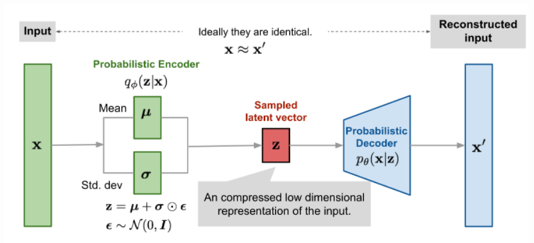

However, this does not completely solve the problem. There may still be gaps in the latent space because the outputted means may be significantly different and the standard deviations may be small. To alleviate this problem, we add an auxilliary loss that penalizes the distribution \(p(z \mid x)\) for being too far from the standard normal distribution \(\mathcal{N}(0, I)\). Let \(J\) be the dimensionality of latent space \(z\). Then, the penalty term is the KL divergence between \(p(z \mid x)\) and \(\mathcal{N}(0, I)\), which is given by

$$

\mathbb{KL}\left( \mathcal{N}(\mu_p, \sigma_p) \parallel \mathcal{N}(\mu_q, \sigma_q) \right) = \sum_{x \in X} \sum_{j \in J} \left(  \log \left( \frac{\sigma_{q_j}}{\sigma_{p_j}} \right) + \frac{\sigma_{p_j}^2 + (\mu_{p_j} - \mu_{q_j})^2}{2 \sigma_{q_j}^2} - \frac{1}{2} \right)

$$

$$

\mathbb{KL}\left( \mathcal{N}(\mu, \sigma) \parallel \mathcal{N}(0, I) \right) = \sum_{x \in X} \sum_{j \in J} \left( \frac{\sigma_{j}^2 + \mu_{j}^2}{2} - \log \sigma_{j} - \frac{1}{2} \right)

$$

You can see the paper(section B) for more detailed derivation of the last formula.

This expression applies to two univariate Gaussian distributions (the full expression for two arbitrary univariate Gaussians is derived in this math.stackexchange post). Extending it to our diagonal Gaussian distributions is not difficult; we simply sum the KL divergence for each dimension.

This loss is useful for two reasons. First, we cannot train the encoder network by gradient descent without it, since gradients cannot flow through sampling (which is a non-differentiable operation). Second, by penalizing the KL divergence in this manner, we can encourage the latent vectors to occupy a more centralized and uniform location. In essence, we force the encoder to find latent vectors that approximately follow a standard Gaussian distribution that the decoder can then effectively decode.

We need to change the Encoder class to produce \(\mu(x)\) and \(\sigma(x)\), and then use these to sample a latent vector. We also use this class to keep track of predicted \(\mu(x)\) and \(\sigma(x)\) to be able to compute KL loss.